Conformal classification using CV+ in a Pipeline

This tutorial demonstrates how to use CoverForestClassifier in a scikit-learn pipeline for CV+ conformal classification on the breast cancer dataset.

import numpy as np
from matplotlib import pyplot as plt
from sklearn import tree
from sklearn.datasets import load_breast_cancer
from sklearn.model_selection import train_test_split
from sklearn.pipeline import Pipeline
from sklearn.preprocessing import StandardScaler

from coverforest import CoverForestClassifier
from coverforest.metrics import average_set_size_loss, classification_coverage_score

Load the dataset and split it into training and testing sets

X, y = load_breast_cancer(return_X_y=True, as_frame=True)
X_train, X_test, y_train, y_test = train_test_split(X, y, test_size=0.2, random_state=0)

Making a pipeline

We’ll create a scikit-learn pipeline that normalizes the features first before fitting with CoverForestClassifier.

pipe = Pipeline(
    [
        ("scaler", StandardScaler()),
        (
            "clf",
            CoverForestClassifier(
                n_estimators=100, method="cv", cv=10, random_state=0, verbose=1
            ),
        ),
    ]
)

We’ll now fit the pipeline on the training data.

pipe.fit(X_train, y_train)

Searching regularization parameters...
Fitting with k = 1 and lambda = 0.1.

Pipeline(steps=[('scaler', StandardScaler()),
                ('clf',
                 CoverForestClassifier(cv=10, n_estimators=100, random_state=0,
                                       verbose=1))])

In a Jupyter environment, please rerun this cell to show the HTML representation or trust the notebook.
On GitHub, the HTML representation is unable to render, please try loading this page with nbviewer.org.

At the default setting, the fit() method performs a hyperparameter search before the actual fitting, which as a result yields k = 1 and lambda = 0.1.

Inspecting individual forest

In constrast to scikit-learn’s RandomForestClassifier, each subestimator in a CoverForestClassifier(method='cv') is a FastRandomForestClassifier, a modification of RandomForestClassifier that skips all input checks for faster training times.

all_forests = pipe["clf"].estimators_
first_forest = all_forests[0]

first_forest

FastRandomForestClassifier(random_state=1162135467)

In a Jupyter environment, please rerun this cell to show the HTML representation or trust the notebook.
On GitHub, the HTML representation is unable to render, please try loading this page with nbviewer.org.

This class retains all RandomForestClassifier’s post-train attributes and methods.

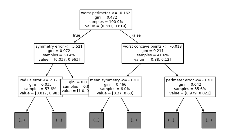
For example, we can plot individual trees in each forest.

plt.figure(figsize=(10, 6))
first_tree = first_forest.estimators_[0]
tree.plot_tree(
    first_tree,
    feature_names=pipe["scaler"].get_feature_names_out(),
    max_depth=2,
    proportion=True,
    fontsize=9,
)
plt.show()

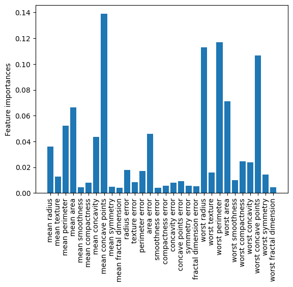
As another example, we plot the feature importances in each forest.

names = pipe["scaler"].get_feature_names_out()
importances = first_forest.feature_importances_

fig, ax = plt.subplots()
ax.bar(names, importances)
ax.set_ylabel("Feature importances")
ax.tick_params(axis="x", labelrotation=90)
plt.show()

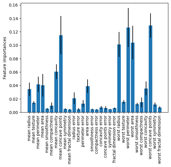
Let’s visualize the variable importances across all forests by plotting the means with 1-sd error bars.

names = pipe["scaler"].get_feature_names_out()
imp_all = [all_forests[i].feature_importances_ for i in range(len(all_forests))]
imp_mean = np.mean(imp_all, axis=0)
imp_std = np.std(imp_all, axis=0)

fig, ax = plt.subplots()
ax.bar(names, imp_mean, yerr=imp_std)
ax.set_ylabel("Feature importances")
ax.tick_params(axis="x", labelrotation=90)
plt.show()

Making set predictions

Now we’ll make predictions with 95% coverage (\(\alpha=0.05\)). This will return both the point predictions and the set predictions.

y_pred, y_sets = pipe.predict(X_test, alpha=0.05)

Here, y_pred is an array of point predictions, which are the single most likely classes predicted by the model. y_sets is a list that contains set predictions.

Let’s compare between the true classes, the single predictions and the set predictions.

for i in range(10, 20):
    print(f"True: {y_test.iloc[i]}, Pred: {y_pred[i]}, Set: {y_sets[i]}")

True: 1, Pred: 0, Set: [0 1]
True: 1, Pred: 1, Set: [1]
True: 1, Pred: 1, Set: [1]
True: 1, Pred: 0, Set: [0 1]
True: 1, Pred: 0, Set: [0 1]
True: 0, Pred: 0, Set: [0 1]
True: 1, Pred: 1, Set: [1]
True: 0, Pred: 0, Set: [0]
True: 0, Pred: 0, Set: [0]
True: 0, Pred: 0, Set: [0]

All test samples with incorrection have both classes in the prediction sets, indicating that the model outputs both classes when they are uncertain about their single predictions.

Evaluations

The coverforest.metrics module provides two metrics for evaluation of set predictions.

• average_set_size_loss calculates the average set size. Small values indicate that our model is quite confident in its predictions.

• classification_coverage_score calculates the *empirical coverage`, that is, the proportion of sets that contain the true classes. Higher coverage scores are better, especially when making risky decisions. The standard guaranteed lower bound on the coverage probability is \(1-2\alpha\). Nonetheless, in practice, a good conformal algorithm should have empirical coverage more than \(1-\alpha\).

print(f"Average set size: {average_set_size_loss(y_test, y_sets)}")
print(f"Empirical coverage: {classification_coverage_score(y_test, y_sets)}")

Average set size: 1.105263157894737
Empirical coverage: 0.9824561403508771

In this particular example, the empirical coverage is above the specified coverage level of 0.982. The average set size of 1.105 indicates that the random forest can output a single label with high confidence.

Comparison with Jackknife+-after-bootstrap and split conformal

Let’s try the remaining two conformal classification methods, namely the Jackknife+-after-bootstrap and split conformal methods and see how they perform compared to CV+.

Jackknife+-after-bootstrap

The model is exactly the same as a regular random forest, but now it keeps track of which samples haven’t been trained by each tree for out-of-bag score calculations.

pipe_b = Pipeline(
    [
        ("scaler", StandardScaler()),
        (
            "clf_b",
            CoverForestClassifier(n_estimators=400, method="bootstrap", random_state=0),
        ),
    ]
)
pipe_b.fit(X_train, y_train)
y_b_pred, y_b_sets = pipe_b.predict(X_test, alpha=0.05)

print(f"Average set size: {average_set_size_loss(y_test, y_b_sets)}")
print(f"Empirical coverage: {classification_coverage_score(y_test, y_b_sets)}")

Average set size: 1.105263157894737
Empirical coverage: 0.9824561403508771

Split conformal

pipe_sp = Pipeline(
    [
        ("scaler", StandardScaler()),
        (
            "clf_sp",
            CoverForestClassifier(n_estimators=400, method="split", random_state=0),
        ),
    ]
)
pipe_sp.fit(X_train, y_train)
y_sp_pred, y_sp_sets = pipe_sp.predict(X_test, alpha=0.05)

print(f"Average set size: {average_set_size_loss(y_test, y_sp_sets)}")
print(f"Empirical coverage: {classification_coverage_score(y_test, y_sp_sets)}")

Average set size: 1.105263157894737
Empirical coverage: 0.9649122807017544

We can see that the split conformal provides a slightly smaller coverage than the other two methods and a larger average set size.

Final notes

1. The methods used for constructing prediction sets are different variations of the adaptive prediction set (APS) method introduced in Romano et al.[1].

2. The CV+ method is the only one with random forests as the sub-estimators

3. The CV+ method also comes with additional parameters, namely:

   • k_init='auto' and lambda_init='auto': Initial regularization parameters

   • allow_empty_sets=True: Whether empty prediction sets are allowed

   • randomized=True: Whether to include one more class to the set prediction at random.

   It is recommended that:

   • If many of the set predictions are empty, it is recommended to increase the target coverage rate (decrease \(\alpha\)) until most sets are nonempty.

   • When allow_empty_sets=False, an additional class is added to all prediction sets, not only the empty ones, due to the exchangeability requirement of conformal prediction. This leads to larger prediction sets overall, so this option should only be used sparingly.

4. In the case of Jackknife+-after-bootstrap, the coverage guarantee in Kim et al.[2] relies on resampling the forest’s tree count from \(\operatorname{Binomial}(B (1-1/n)^m)\), where:

   • \(B\) is the initial number of trees

   • \(n\) is the number of training samples

   • \(m\) is the number of bootstrap samples.

   The fit() method in CoverForestClassifier automatically sets \(B= \text{n_estimators}/(1-1/n)^m\) so that, on average, the number of trees to be fitted is \(\text{n_estimators}\), with standard deviation of \(\sqrt{\text{n_estimators}*(1- (1-1/n)^m)}\).

   CoverForestClassifier also provides an option not to resample the number of sub-estimators by initiating with resample_n_estimators=False.

5. Random forest leverages parallel computation by processing trees concurrently. Use the n_jobs parameter in fit() and predict() to control CPU usage (n_jobs=-1 uses all cores).

6. For prediction, conformity score calculations require a memory array of size (n_train × n_test × n_classes). To optimize performance with high n_jobs values, split large test sets into smaller batches.

---

[1]

Yaniv Romano, Matteo Sesia, and Emmanuel Candes. Classification with valid and adaptive coverage. In H. Larochelle, M. Ranzato, R. Hadsell, M.F. Balcan, and H. Lin, editors, Advances in Neural Information Processing Systems, volume 33, 3581–3591. Curran Associates, Inc., 2020. URL: https://proceedings.neurips.cc/paper_files/paper/2020/file/244edd7e85dc81602b7615cd705545f5-Paper.pdf.

[2]

Byol Kim, Chen Xu, and Rina Barber. Predictive inference is free with the jackknife+-after-bootstrap. In H. Larochelle, M. Ranzato, R. Hadsell, M.F. Balcan, and H. Lin, editors, Advances in Neural Information Processing Systems, volume 33, 4138–4149. Curran Associates, Inc., 2020. URL: https://proceedings.neurips.cc/paper_files/paper/2020/file/2b346a0aa375a07f5a90a344a61416c4-Paper.pdf.