Searching \(k\) and \(\lambda\) using scikit-learn’s GridSearchCV

The parameter \(k\) is essentially the upper limit on the sizes of the prediction sets. Thus, by its definition, we should choose \(k\) so that the true class \(y\) are within the top-\(k\) most likely classes for most samples. Specifically, if we want our prediction set to contain the true class \((1-\alpha)\%\) of the time, a suitable choice of \(k\) is the (\(1-\alpha\)) quantile of the ranks of the true classes based on their predicted probabilities, from highest to lowest.

The CoverForestClassifier class provides the search_k_and_lambda() method that searches for \(k\) using the method described in the previous paragraph; while \(\lambda\) is chosen from the candidates \(0.001, 0.01, 0.1, 0.2, 0.5, 1\) using cross-validation. In this tutorial, we will instead use the grid-search functionality provided by scikit-learn to search for \(k\) and \(\lambda\) over any choice of search spaces.

This tutorial demonstrates how to perform grid-search cross-validation for CoverForestClassifier’s \(k\) and \(\lambda\) parameters on the MNIST dataset.

import numpy as np
from matplotlib import pyplot as plt
from sklearn.datasets import load_digits
from sklearn.metrics import make_scorer
from sklearn.model_selection import GridSearchCV, train_test_split

from coverforest import CoverForestClassifier
from coverforest.metrics import average_set_size_loss

Load the dataset and take a look at the first few images.

digits = load_digits()

_, axes = plt.subplots(nrows=1, ncols=4, figsize=(10, 3))
for ax, image, label in zip(axes, digits.images, digits.target):
    ax.set_axis_off()
    ax.imshow(image, cmap=plt.cm.gray_r, interpolation="nearest")
    ax.set_title("Training: %i" % label)

We’ll split the data into 50% training and 50% testing sets

X_train, X_test, y_train, y_test = train_test_split(
    digits.data, digits.target, test_size=0.5, shuffle=False
)

Limiting the search space

When dealing with problems that have many possible classes, searching through all possible values of \(k\) (from 1 up to the total number of classes) would be computationally expensive. Instead, we can narrow down the search range for \(k\) using the quantile-based approach described at the beginning. In particular, we will use the search_k_and_lambda() method, which will output a particular value of \(k\), then we will limit our search space to integers near this value.

To search for \(k\), we specify k_init="auto" and lambda_init=0. We also setalpha_default=0.05 which will not be used for now, but it will be used when GridSearchCV calls clf’s predict() method during fitting.

clf = CoverForestClassifier(
    n_estimators=100,
    method="cv",
    cv=5,
    k_init="auto",
    lambda_init=0,
    alpha_default=0.05,
    random_state=0,
)
clf.search_k_and_lambda(X_train, y_train)

(1, 0)

We obtain \(k=1\). From this, we will perform grid-search cross validation with \(k\) ranging from \(1\) to \(3\) and \(\lambda\) from \(0.001\) to \(10\).

param_grid = {"k_init": [1, 2, 3], "lambda_init": [0.001, 0.01, 0.1, 1.0, 10.0]}

average_set_size_score = make_scorer(average_set_size_loss, greater_is_better=False)

grid_search = GridSearchCV(
    clf, param_grid, cv=5, scoring=average_set_size_score, n_jobs=-1
)

grid_search.fit(X_train, y_train)

print(f"Best parameters: {grid_search.best_params_}")
print(f"Best score: {grid_search.best_score_:.3f}")

Best parameters: {'k_init': 1, 'lambda_init': 1.0}
Best score: -1.922

From the grid-search, the best parameters are \(k=1\) and \(\lambda=1.0\) which yield the smallest average set size of \(1.922\).

Comparison between models with and without regularization

Let’s see if the regularization actually improve the model in terms of average set size.

First, we fit another model without regularization (\(k=0\) and \(\lambda=0\)).

another_clf = CoverForestClassifier(
    n_estimators=100, method="cv", cv=5, k_init=0, lambda_init=0, random_state=0
)
another_clf.fit(X_train, y_train)
y_pred, y_sets = another_clf.predict(X_test, alpha=0.05)

contain_y = [y_test[i] in y_sets[i] for i in range(len(y_test))]
set_sizes = [len(s) for s in y_sets]
print(f"Test coverage: {np.mean(contain_y):.3f}")
print(f"Average set size: {np.mean(set_sizes):.3f}")

Test coverage: 0.970
Average set size: 2.241

Let’s compare the result to that of our grid-searched model.

best_clf = grid_search.best_estimator_
y_pred, y_sets = best_clf.predict(X_test, alpha=0.05)

contain_y = [y_test[i] in y_sets[i] for i in range(len(y_test))]
set_sizes = [len(s) for s in y_sets]
print(f"Test coverage: {np.mean(contain_y):.3f}")
print(f"Average set size: {np.mean(set_sizes):.3f}")

Test coverage: 0.970
Average set size: 2.004

In this example, the regularization actually helps decrease the average set size.

Inspecting a difficult image

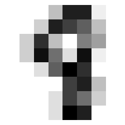
Let’s now take a look at an image with the largest prediction set.

print(f"Largest set size: {max(set_sizes)}")

Largest set size: 7

Below, we plot a test image whose prediction set has seven classes.

idx = set_sizes.index(7)

img_idx = X_test[idx].reshape(8, 8)

_, ax = plt.subplots(figsize=(3, 3))
ax.set_axis_off()
ax.imshow(img_idx, cmap=plt.cm.gray_r, interpolation="nearest");

This is most likely a 9, a 5 or an 8 might be possible. Let’s see the model’s set prediction.

print(f"True class: {y_test[idx]}")
print(f"Single prediction: {y_pred[idx]}")
print(f"Set prediction: {y_sets[idx]}")

True class: 8
Single prediction: 9
Set prediction: [0 1 3 5 7 8 9]